Models
Contents
Baseline Algorithm
Our baseline model will be an unsupervised learning model as we do not have labeled data. First, we split the playlists into a train and test set using a 80-20 split, such that 80% of the total number of playlists form the training data and 20% form the test data. From the EDA, we observed the high pairwise correlation between energy, acousticness, and loudness, thus because of in our model we will keep just one of these parameters. We chose energy as it has the largest correlation with the other two. The other parameters were duration_ms, liveness, instrumentalness, danceability, key, mode, valence, tempo, and popularity. We now focus on the training set and use our k-means clustering algorithm to label playlists as belonging to one of 4 clusters.
Having now obtained labeled data, we train a Random Forest with number of trees equal to 50 and maximum depth equal to 20 to match songs to their respective playlist cluster. While this is somewhat circular as we have used the k-means algorithm to label the data and we are now finding classes within the our own label data, it allows us to verify if our model makes sense and if it is performing well on our simplistic labeled data. We point that on the other end of the scale would be to allow each to be its own separate class, but this would likely lead to an intractable problem where the algorithm will either only work on large playlists or where it will not work at all. Some fancy bootstrap-like technique might provide salvation for the short playlists, but either way, we believe that allowing each playlist to be its own separate class will lead to over-fitting.
We then evaluate our algorithm (the mix of k-means and Random Forest) on the train set and obtain a score of 0.993, while on the test set we obtain a score of 0.612. Of course there is a lot of improvements possible. One idea would be to focus only on large playlists and split them in training and test set song, and use Random Forest (or other classifier) on the training set. We would then use a large data base of songs and see what are the top predictions for songs (where the top prediction number equals the test set number of songs) and how many of these predictions are actually present in the test set.
MinMax Algorithm
Assumptions
We make an assumption that playlists often serve a purpose of accompanying a specific event. It helps set the tone and mood of an activity. Users create playlists for specific moods such as working out, partying, studying, and sleeping. For instance, a user that may be throwing a party would want to play a sequence of upbeat music. It would feel out of place for the guests to listen to a playlist full of classical music.
Our second assumption relies on the nature of music that different genres of music embody different features. For instance, we expect indie music to have high acousticness and low danceability. For simplicity, we assume that each genre has a maximizing and minimizing feature.
Algorithm
We design an algorithm such that it generates playlists based on the mood specified by the user. The algorithm takes in two features - one that the user wants to maximize and another that the user wants to minimize. We can use the two features as a proxy for the "mood" of the playlist.
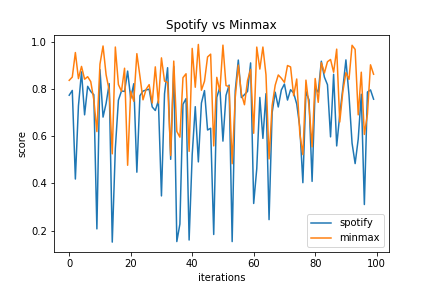
From our original data set containing 1,000,000 playlists, we randomly choose 1000 playlists as our pool of songs. We then cluster the pool of songs using the KMeans algorithm. We randomize the number of clusters to be in between [4, 10]. For each cluster, we choose the top n songs with the highest values for the feature that the user wants to maximize. We define n as the number of songs in the playlist that yields to the best score in the Spotify data. We use the bootstrap method by running the KMeans algorithm 10 times, and choosing the playlist that yields to the best score. We define the formla for the best score below.
Evaluation Metric
To define the evaluation metric for the playlists, we rely on the assumption that the playlist that reflects the best maximizing and minimizing features yields to the best user satisfaction. To compute the score of a playlist based on the maximizing and minimizing features, we take the difference between the mean of the two features. More concretely, if we have 2 playlists:
- Playlist 1 has 3 songs with (1, 1, 1) and (0, 0, 0) for danceability and acousticness respectively.
- Playlist 2 has 3 songs with (0, 0, 0) and (1, 1, 1) for danceability and acousticness respectively.
Results
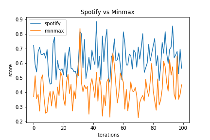
Setting the maximizing feature as danceability and minimizing feature as acousticness, we compare the playlist generated by MinMax on the left to the playlist generated by Spotify on the right.
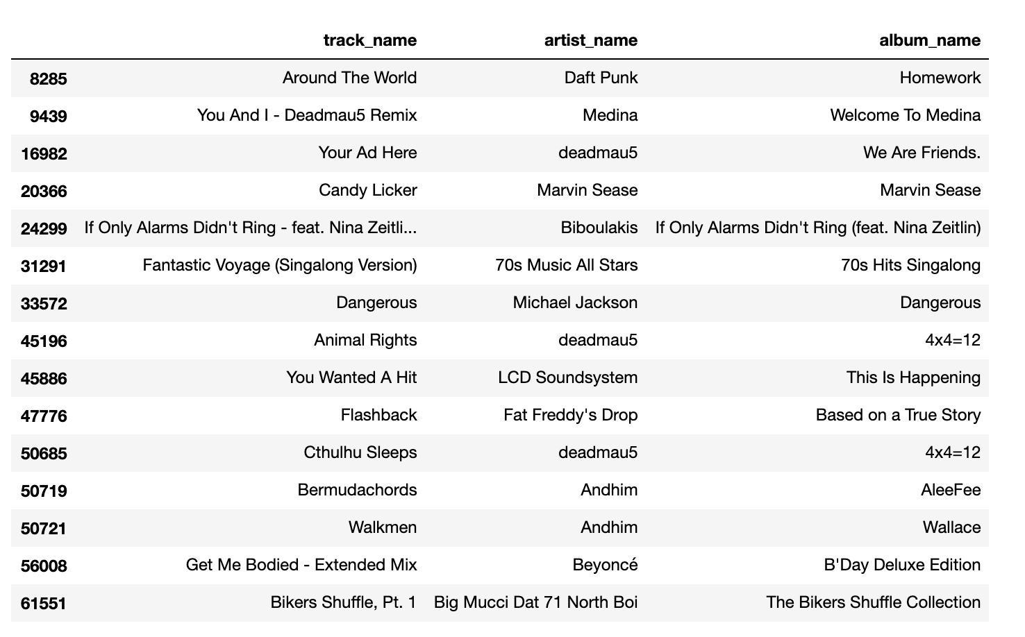
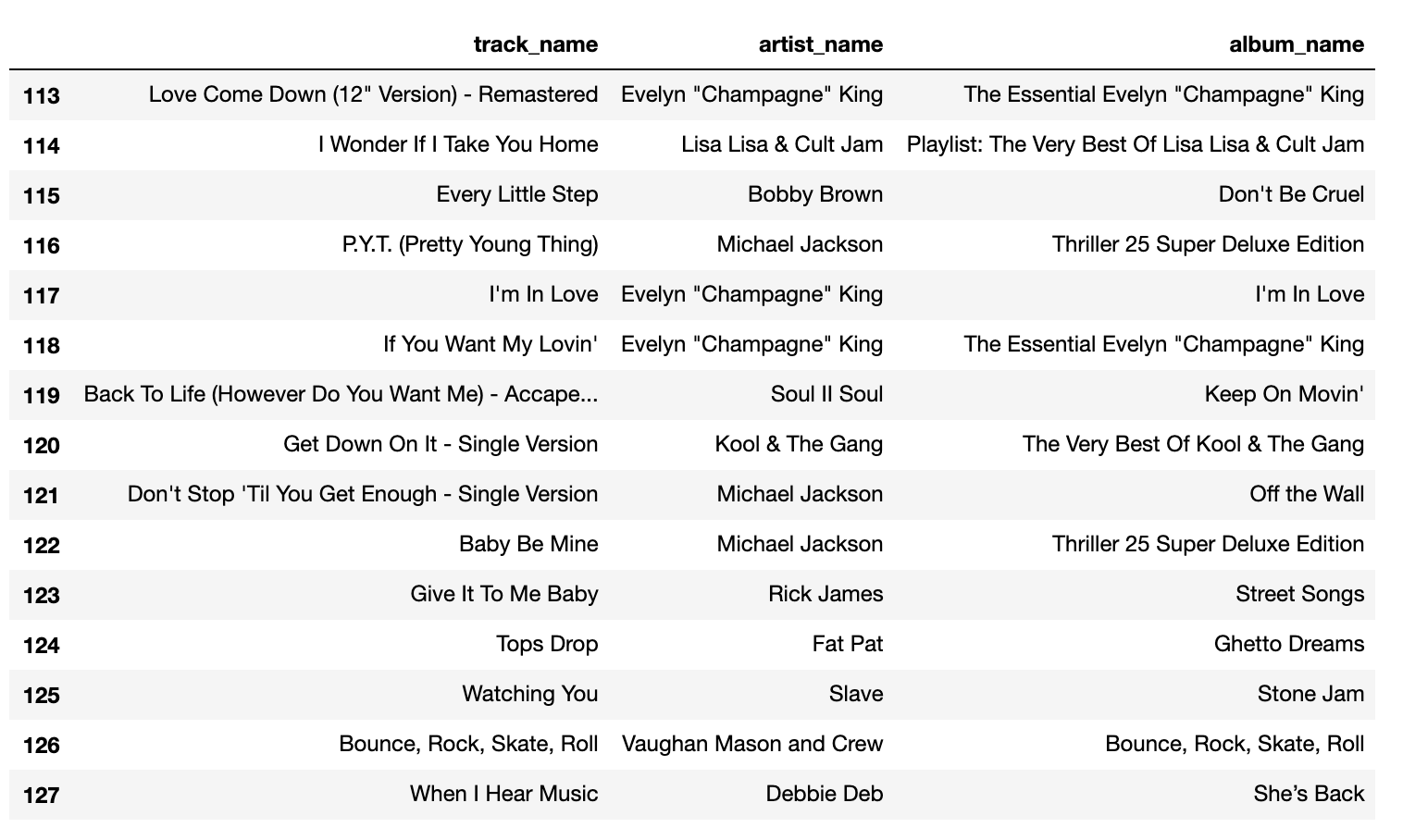
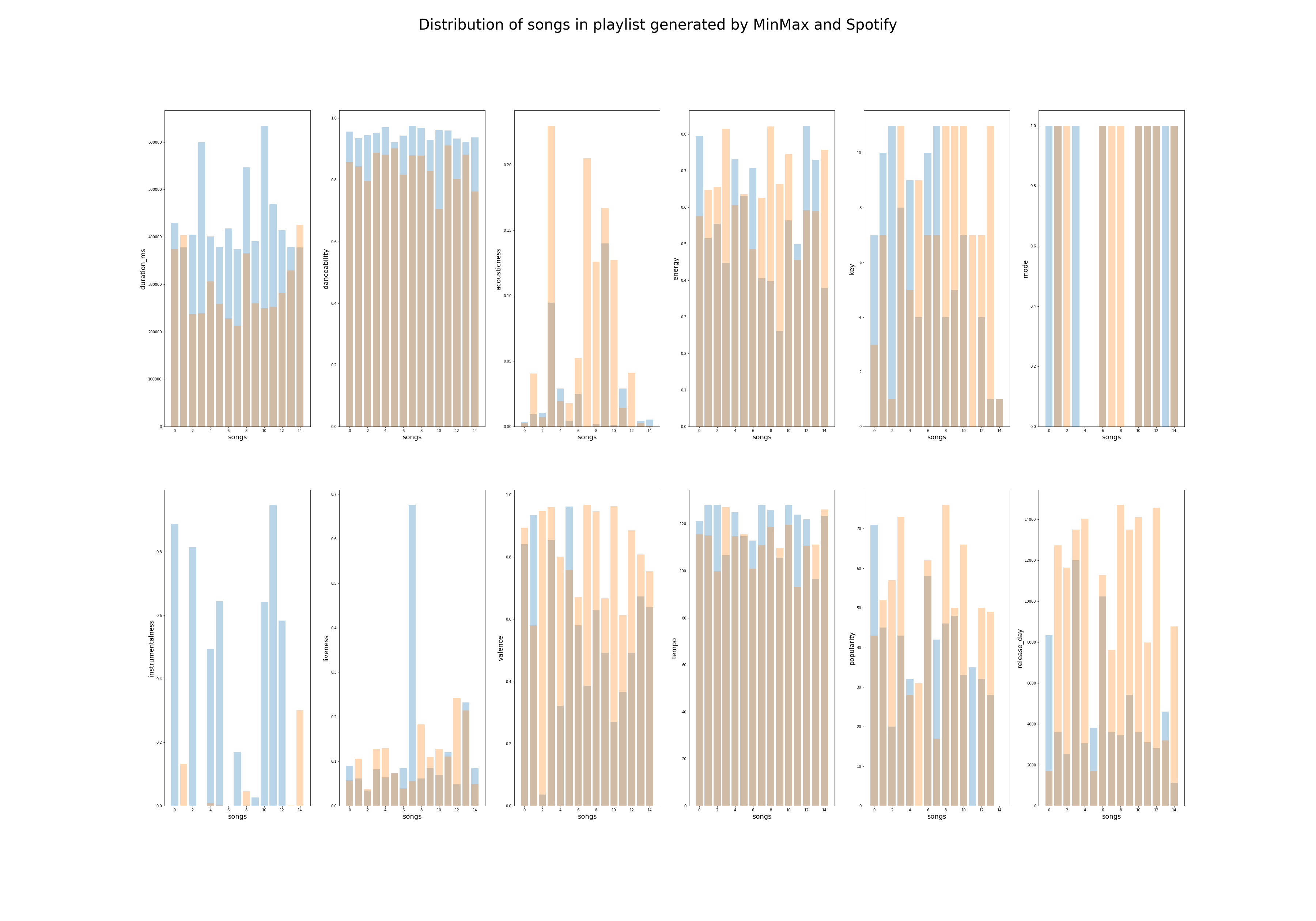
The playlist generated by MinMax and Spotify have some songs that are similar. There are overlapping 70's music in both playlists. In the MinMax playlist, however, we see pop and edm artists such as Beyonce and deadmau5. To analyze the results further, the distribution of features for each playlist is shown below,
Song Seed Algorithm
Assumptions
We assume that the average parameters of a playlist (such as duration_ms, danceability, etc.) are representative of the type of playlist. We then use a 10-dimensional space given by the most important and least correlated features of a song (as we discovered in the EDA). These are duration_ms, danceability, energy, key, mode, instrumentalness, liveness, valence, tempo, and popularity. For a given playlist, we average these parameters out and depict the playlist by one point, which we assume is good representation of our playlist. We assume that the closer two such data points are to each other, the more similar the playlists.
Algorithm
First, we split the playlists into a train and test set using a 80-20 split, such that 80% of the total number of playlists form the training data and 20% form the test data. We then represent each training playlist by one data point in our 10-dimensional space. From the EDA, we saw that using k-means with 4 clusters is a good choice to separate our data, however given the highly dense dataset we might decided to increase the number of clusters to 100, such that very similar playlists are grouped together more closely. Note, we acknowledge that this 100 clusters are arbitrary and in the future we should likely look at a way to better select this value. However, we also would like to point out that there were no clearly defined clusters as our playlists occupied rather continuously in the 10-dimensional subspace (selecting the k in k-means in this conditions can be arbitrary as the elbow method for example does not show a clear elbow). More importantly, we use such a high cluster number for speeding up our algorithm and the time it takes to find similar playlists. We explain this in detail below.
We use the 100-means clustering algorithm to assings our playlists (and the songs the contain) to the 100 clusters. Note that one playlist belongs exclusively to one cluster, however a song can belong to multiple clusters and can have multiple instances for a cluster. We now select a playlist from the test set and using a 60-40 split we create a seed playlist (60% of the songs in the selected test playlist) and test songs (40% of the songs in the selected test playlist). Based on the seed playlist, we determine to which of the 100 clusters it belongs. Once this is determined, we look for playlists (the training one that were previously assigned) within this cluster that show the largest overlap in songs with the seed playlist. A typical value that we considered for the minimum number of songs overlapping was 5. This value was chosen as tradeoff between the speed of the code and accuracy of the predictions as defined below. Once these playlists have been determined we then list all the songs that were part of these playlist, but not a member of the seed playlist. We refer to these songs as forming the possibility pool. The most frequently occurring songs in the possibility pool are the ones we use as predictions to add our seed playlist. The total number of songs predicted is of course equal to number of test songs.
Evaluation Metrics and Results
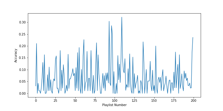
We evaluate our algorithm in three ways. First, we calculate the ratio of correct predictions to the total number of songs predicted; we call this accuracy. A plot of it is shown below. We notice that the average is 7%, which in all fairness is not great but is much better than an average chance prediction by a couple of orders of magnitude. We also see that at times it reaches above 30%.
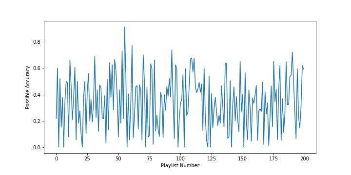
Second, we calculate the ratio between the number of songs in the possibility pool that overlap with the test songs and the total number of test songs. We refer to this as the possible accuracy and we show a plot of it below. We notice that the average is 34%, which again in all fairness is still not ideal but also almost 5 times better than our accuracy. We also see that at times the possible accuracy reaches above 80%.
Third, we compute the time it took to run our algorithm on an average computer. For 200 test playlists of around 200 songs each, the algorithm took an hour to perform predictions. A faster computer and likely an optimised code would decrease this time as it is taking rather long to perform this predictions.
Overall, our algorithm is performing much better than random chance but it is unlikely that Spotify will be using our implementation.